First-Order Homogeneous Equations
A function f( x,y) is said to be homogeneous of degree n if the equation
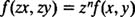
holds for all x,y, and z (for which both sides are defined).
Example 1: The function f( x,y) = x 2 + y 2 is homogeneous of degree 2, since

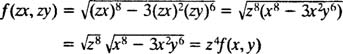
Example 2: The function 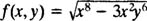 is homogeneous of degree 4, since
Example 3: The function f( x,y) = 2 x + y is homogeneous of degree 1, since

Example 4: The function f( x,y) = x 3 – y 2 is not homogeneous, since

which does not equal z n f( x,y) for any n.
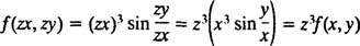
Example 5: The function f( x,y) = x 3 sin ( y/x) is homogeneous of degree 3, since
A first‐order differential equation  is said to be homogeneous if M( x,y) and N( x,y) are both homogeneous functions of the same degree.
Example 6: The differential equation
is homogeneous because both M( x,y) = x 2 – y 2 and N( x,y) = xy are homogeneous functions of the same degree (namely, 2).
The method for solving homogeneous equations follows from this fact:
The substitution y = xu (and therefore dy = xdu + udx) transforms a homogeneous equation into a separable one.
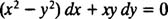
Example 7: Solve the equation ( x 2 – y 2) dx + xy dy = 0.
This equation is homogeneous, as observed in Example 6. Thus to solve it, make the substitutions y = xu and dy = x dy + u dx:
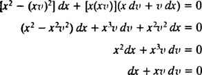
This final equation is now separable (which was the intention). Proceeding with the solution,
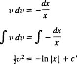
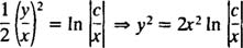
Therefore, the solution of the separable equation involving x and v can be written

To give the solution of the original differential equation (which involved the variables x and y), simply note that
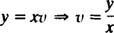
Replacing v by y/ x in the preceding solution gives the final result:
This is the general solution of the original differential equation.
Example 8: Solve the IVP
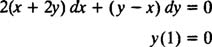
Since the functions

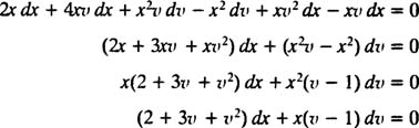
are both homogeneous of degree 1, the differential equation is homogeneous. The substitutions y = xv and dy = x dv + v dx transform the equation into

which simplifies as follows:
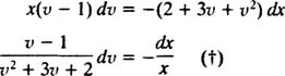
The equation is now separable. Separating the variables and integrating gives
The integral of the left‐hand side is evaluated after performing a partial fraction decomposition:
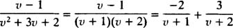
Therefore,
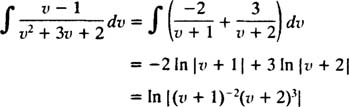
The right‐hand side of (†) immediately integrates to
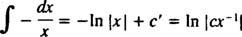
Therefore, the solution to the separable differential equation (†) is
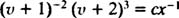
Now, replacing v by y/ x gives
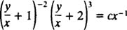
as the general solution of the given differential equation. Applying the initial condition y(1) = 0 determines the value of the constant c:
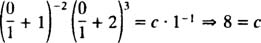
Thus, the particular solution of the IVP is
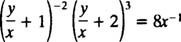
which can be simplified to
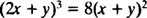
as you can check.
Technical note: In the separation step (†), both sides were divided by ( v + 1)( v + 2), and v = –1 and v = –2 were lost as solutions. These need not be considered, however, because even though the equivalent functions y = – x and y = –2 x do indeed satisfy the given differential equation, they are inconsistent with the initial condition.